This package is a forward simulator designed to generate synthetic metacommunity data. As an in silico experimental platform, it enables researchers to computationally generate hypothetical community shifts, test theoretical frameworks and benchmark analytical algorithms prior to empirical application.
Core capabilities include:
- Mechanistic simulation: Generates spatially explicit community dynamics driven by local demography, dispersal, and interspecific interactions.
-
GIS interoperability: Built on the
terraecosystem, the package reads and writes standard spatial formats (such as GeoTIFFs and ESRI grids), allowing simulations to run across dynamic environments. - Virtual ecologist module: Bridges the gap between theory and empirical data by applying a hierarchical observation layer to the generated ground truth. Users can explicitly simulate imperfect detection and abundance estimation errors to mimic real-world biodiversity surveys.
Basic Workflow
The mrangr workflow involves initialising a community with spatial data and interaction parameters, running the simulation, and analysing the results.
1. Input Maps and Interactions
You must provide carrying capacity maps (K_map) and initial abundance maps (n1_map) as SpatRaster objects. For a community of species, the rasters must contain layers.
# Load example maps
K_map <- rast(system.file("input_maps/K_map_eg.tif", package = "mrangr"))
K_map <- subset(K_map, 1:2)
Interspecific interactions are defined using an interaction matrix (), where values represent the per-capita interaction strength of the species in the column on the species in the row.
2. Community Initialisation
Use initialise_com() to create a sim_com_data object. This stores all parameters, including the intrinsic growth rate () and the dispersal rate.
first_com <- initialise_com(
  n1_map = round(K_map / 2),
  K_map = K_map,
  r = 1.1,
  a = a,
  rate = 1 / 500
)
3. Running the Simulation
The sim_com() function executes the simulation over a specified number of time steps.
first_sim <- sim_com(first_com, time = 100)4. Visualisation
You can visualise the final spatial distributions or the change in mean abundance over time.
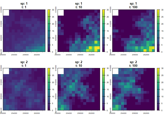
# Plot abundance time series for all species
plot_series(first_sim)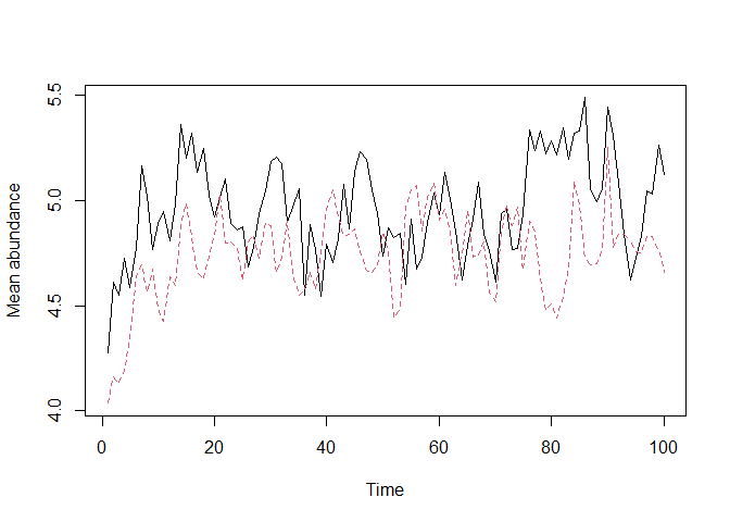
Virtual Ecologist
The package includes a virtual_ecologist() function to simulate real-world observation processes. This allows users to sample the simulated community at defined points in space and time, incorporating sampling effort and detection probability into the simulation.